“When the term machine is used in ordinary discourse, it tends to
evoke an unattractive picture. It brings to mind a big, heavy,
complicated object which is noisy, greasy, and metallic; performs jerky
repetitive, and monotonous motions; and has sharp edges that may hurt
one if he does not maintain sufficient distance… Our concern is with
questions about the ultimate theoretical capacities and limitations of
machines [and so] it is necessary to abstract away many realistic
details and features of mechanical systems…
We ignore, in our abstraction, the geometric or physical composition of
mechanical parts. We ignore questions about energy. We even shred time
into a sequence of separate, disconnected moments, and we totally ignore
space itself! Can such a theory be a theory of any ‘thing’ at all?
Incredibly, it can indeed.” - Marvin Minsky, Computation: Finite and
Infinite Machines
Our fundamental model of computation in this class will be the
state machine.
A state machine is (a formal specification of) any system that can be
in different states/configurations at different times, and which can
change its state/configuration depending on external events (user input,
time passing, etc.).
Example
Most notably, any modern digital computer is a state machine. The
“state” of the machine at any instant includes the state of all the bits
in memory, the bits on the disk, the bits in CPU registers, etc. As
computation progresses, the CPU changes these bits, and the system
transitions from one state to the next.
A computer game can be viewed as a state machine. The state of the
system includes all the information about the current game state, e.g.,
the current level, the position and possibly velocity of the player and
other game entities, and (in general) any information that we’d need to
remember in order to resume the game if the user wants to temporarily
pause the game and continue it at a later time. How the state changes
depends on the passage of time and the player’s actions.
A vending machine can be viewed as a state machine. The state of the
system includes (at least) the number and position of the items being
sold, the contents and capacity of the change collection and dispensing
units. In normal circumstances, this system changes its state only when
customers interact with the machine.
Deterministic State Machines
We say that a state machine is deterministic if, given the
current state and an external event, there is a unique next
state (determined by the current state and the specific event) of the
system. More formally:
Definition
A Deterministic State Machine is a 5-tuple \((Q, \Sigma, \delta, q_0, F)\) where >
>- \(Q\) is a nonempty set.
> The elements of \(Q\) are called
states; each corresponds to a potential configuration of the machine.
>- \(\Sigma\) is an alphabet (a
nonempty finite set).
> Elements of \(\Sigma\) represent
possible events or inputs. >- \(\delta : Q
\times \Sigma \to Q\) is the transition function.
> A system in state \(q\) that sees
input \(a\) will change its state to
\(\delta(q,a)\). >- \(q_0 \in Q\) is the start state.
>- \(F \subseteq Q\) is the set of
final (or accepting) states.
Definition
We say that a deterministic state machine \(M=(Q, \Sigma, \delta, q_0, F)\)accepts a string \(w\in\Sigma^*\) if following transitions
(using \(\delta\)) starting from \(q_0\) according to the successive letters
of \(w\) we end up in a state in \(F\). > More formally, \(M\)accepts a string \(w\in\Sigma^*\) if \(\mathsf{accept}(q_0, w)\) is true, where
the \(\mathsf{accept}\) predicate is
defined recursively as follows: >\[
>\begin{array}{lcl}
> \mathsf{accept}(q, \epsilon) & \mathrm{if}
& q\in F \\
> \mathsf{accept}(q, aw ) & \mathrm{if} &
\delta(q, a) = q' \mathrm{\ and\ } \mathsf{accept}(q', w)\\
> \end{array}
>\] >Given a state machine \(M\), its language\(L(M)\) is defined to be the set of all
strings accepted by the machine, i.e., >\[
>L(M) := \{\ w\in\Sigma^*\ |\ \mathsf{accept}(q_0, w)\ \}.
>\] It follows that \(M\)
accepts \(w\) iff \(w\in L(M)\).
DFAs
Definition
A Deterministic Finite State Machine (DFSM), also known as a
Deterministic Finite Automaton (DFA), is a deterministic state
machine \(D=(Q, \Sigma, \delta, q_0,
F)\) where the set of possible states \(Q\) is finite.
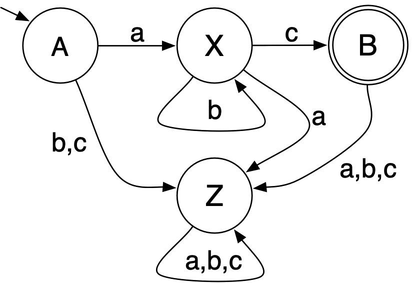
Example
For small DFAs, it’s common to specify the components of the state
machine visually: > > > >- The states are represented by
circles, so \(Q =\{A,X,B,Z\}\) >-
The alphabet is the labels of the arrows, so \(\Sigma = \{a,b,c\}\) >- The arrows show
the transition relation, so \(\delta(A,a)=X\), \(\delta(A,b)=Z\), \(\delta(X,b)=X\), etc. >- The start state
has an extra incoming arrow, so \(q_0 =
A\) >- States drawn with a double circle are final, so \(F = \{B\}\)
Example
This same DFA > > >- does not accept abb,
because the transitions take us from the start state \(A\) to \(X\) to \(X\) to \(X\), and \(X\) is not an accepting state. >- does
accept abc, because the transitions take us from \(A\) to \(X\) to \(X\) to \(B\), and \(B\) is an accepting state. >- does not
accept abca, because the transitions take us from \(A\) to \(X\) to \(X\) to \(B\) to \(Z\), and \(Z\) is not an accepting state.
Example
A two-state DFA
This DFA accepts any string of 0’s and 1’s that contains an even
number of 0’s (by using different states to keep track of whether it has
seen an even number of 0’s so far, or an odd number of 0’s).
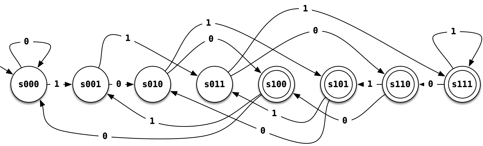
Example
An eight-state DFA
This DFA accepts any string in which 1 is the third to last character
(by using different states to keep track of the three most-recently seen
bits).
Nondeterministic Finite
Automata (NFAs)
It can be useful to relax the requirement that our finite state
machines be deterministic. A Nondeterministic Finite State
Machine (NDFSM) or Nondeterministic Finite Automaton (NFA)
allows a choice of possible next states for a given input, and it allows
a change of state even in the absence of inputs. Further, given such a
choice, an NFA can correctly “guess” which transition to take next!
Guessing is hard to implement directly, but we’ll see later that it’s
possible to implement indirectly because any NFA can be simulated by a
DFA (and hence, in principle, by a digital computer).
Definition
An NFA (Nondeterministic Finite Automaton) is a 5-tuple \((Q, \Sigma, \delta, q_0, F)\) where >
>- \(Q\) is a nonempty
finite set of states. >- \(\Sigma\) is an alphabet. >- \(\delta : (Q\cup\{\epsilon\}) \times \Sigma \to
{\cal{P}}(Q)\) is the transition function.
> \({\cal{P}}(Q)\) is the powerset
of \(Q\), the collection of all subsets
of \(Q\).
> If the system is in state \(q\)
and sees input \(a\), it can change its
state to one of the elements of \(\delta(q,a)\). Alternatively, if the system
is in state \(q\) it can spontanously
transtition to any state in \(\delta(q,\epsilon)\) without seeing any
input. >- \(q_0 \in Q\) is the
start state. >- \(F \subseteq
Q\) is the set of final (or accepting)
states.
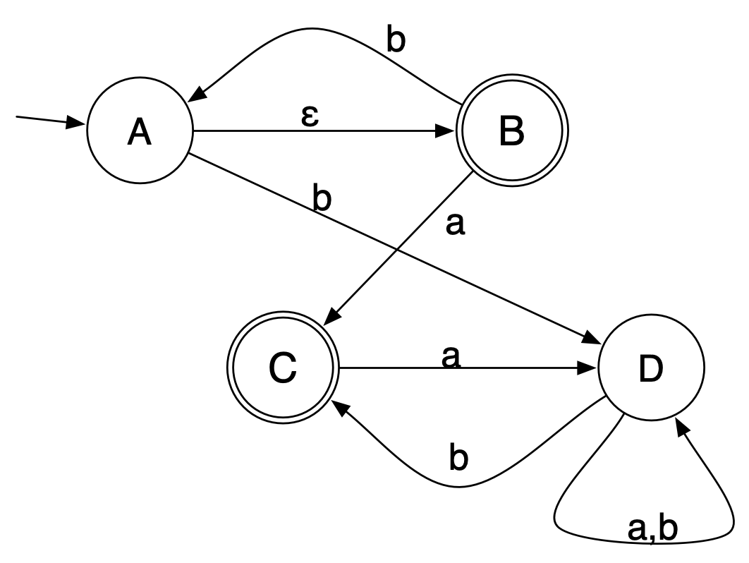
Example
For small NFAs, it’s common to specify the components of the state
machine visually: > > >- The states are represented by
circles, so \(Q = \{A,B,C,D\}\) >-
The alphabet is the labels of the arrows (other than \(\epsilon\)), so \(\Sigma = \{a,b\}\) >- The arrows show
the transition relation, so \(\delta(A,a)=\emptyset\), \(\delta(A,b)=\ D\}\), \(\delta(A,\epsilon)=\{B\}\), …, \(\delta(D,a)=\{D\}\), \(\delta(D,b)=\{C,D\}\), \(\delta(D,\epsilon)=\emptyset\). >- The
start state has an extra incoming arrow, so \(q_0 = A\) >- States drawn with a double
circle are final, so \(F =
\{B,C\}\)
Definition
An NFA \(N = (Q, \Sigma, \delta, q_0,
F)\)accepts the string \(w\in\Sigma^*\) if it is possible
to take transitions spelling out \(w\)
(plus optionally transitions labeled \(\epsilon\) and get from the start state
\(q_0\) to some accepting state in
\(F\). > The language \(L(N)\) of NFA \(N\) is the set of strings accepted by \(N\).
Example
This same NFA > > > >- accepts bb via the
path \(A\), \(D\), \(C\). > > Note: it doesn’t matter that
there are other paths spelling out bb that don’t accept,
such as \(A\), \(D\), \(D\); an NFA accepts if at all possible, so
as long as one accepting path exists, the string is accepted! >-
accepts b via the path \(A\), \(B\)
(via \(\epsilon\)), \(A\), \(B\)
(via \(\epsilon\) again). > >
This path spells out \(\epsilon b
\epsilon\), but that’s just the same string as \(b\), because a string doesn’t change when
you append an empty string. > - accepts aaab via the
path \(A\), \(B\) (via \(\epsilon\)), \(C\), \(D\), \(C\). >- accepts ba via the
path \(A\), \(B\) (via \(\epsilon\)), \(A\), \(B\)
(via \(\epsilon\) again), \(C\). >- does not accept aa
because there is no path from \(A\) to
an accepting state that involves two a transitions (even
allowing \(\epsilon\) transitions).
Example
NFAs can be much smaller than the equivalent DFA. To determine
whether the third-to-last digit of a binary input is 1, the DFA above
required eight states. An NFA can do the same job in four states: >
> This NFA
stays until the start state until all but the last three bits have been
read; if the third-to-last bit is a 1, it can then transition to an
accept state. > If we wanted to know the fourth-to-last digit, a DFA
would require 16 states, whereas an NFA would require only five. If we
wanted the fifth-to-last digit, a DFA would require 32 states, whereas
an NFA would require only six. In general, DFAs can be exponentially
bigger than NFAs to do the same job.
Soon we will show that for any DFA there is a NFA with the same
language, and vice-versa. But first, we need to define the notion of a
Regular Language.
 > >- The states are represented by
circles, so \(Q =\{A,X,B,Z\}\) >-
The alphabet is the labels of the arrows, so \(\Sigma = \{a,b,c\}\) >- The arrows show
the transition relation, so \(\delta(A,a)=X\), \(\delta(A,b)=Z\), \(\delta(X,b)=X\), etc. >- The start state
has an extra incoming arrow, so \(q_0 =
A\) >- States drawn with a double circle are final, so \(F = \{B\}\)
> >- The states are represented by
circles, so \(Q =\{A,X,B,Z\}\) >-
The alphabet is the labels of the arrows, so \(\Sigma = \{a,b,c\}\) >- The arrows show
the transition relation, so \(\delta(A,a)=X\), \(\delta(A,b)=Z\), \(\delta(X,b)=X\), etc. >- The start state
has an extra incoming arrow, so \(q_0 =
A\) >- States drawn with a double circle are final, so \(F = \{B\}\)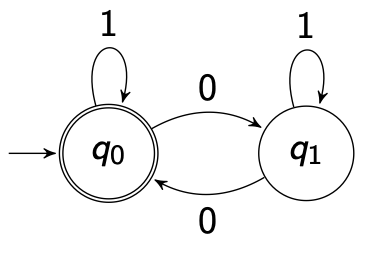
 > >- The states are represented by
circles, so
> >- The states are represented by
circles, so 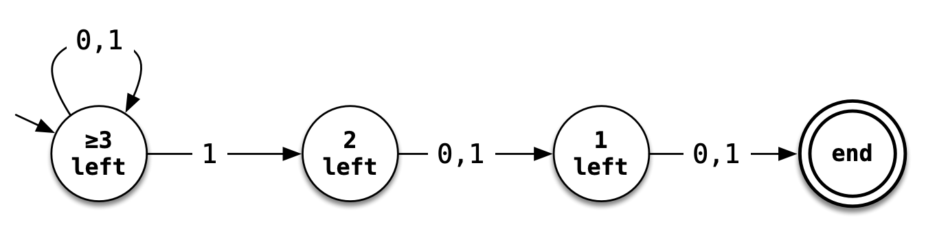 > This NFA
stays until the start state until all but the last three bits have been
read; if the third-to-last bit is a 1, it can then transition to an
accept state. > If we wanted to know the fourth-to-last digit, a DFA
would require 16 states, whereas an NFA would require only five. If we
wanted the fifth-to-last digit, a DFA would require 32 states, whereas
an NFA would require only six. In general, DFAs can be exponentially
bigger than NFAs to do the same job.
> This NFA
stays until the start state until all but the last three bits have been
read; if the third-to-last bit is a 1, it can then transition to an
accept state. > If we wanted to know the fourth-to-last digit, a DFA
would require 16 states, whereas an NFA would require only five. If we
wanted the fifth-to-last digit, a DFA would require 32 states, whereas
an NFA would require only six. In general, DFAs can be exponentially
bigger than NFAs to do the same job.